Recently, we've been looking at different ways to take information from one column and split it out into two or more columns. We used the example of a full name column that we wanted to separate into first and last names. We explored how to split columns using, Power Query, Text to Columns, Formulas, and Flash Fill.
Today's tutorial is inspired by comments from Prof YC and Mohamad on our YouTube channel asking if we can do the opposite.
1. Formula Using Ampersand (&)
Compatibility: All versions of Excel on all operating systems.
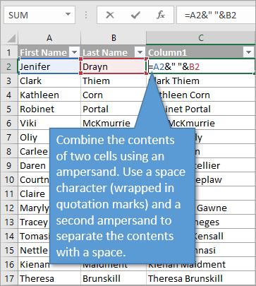
The first way to go about combining text is by using a simple formula. To join cells together we use the ampersand symbol (&). Joining the contents of cells A2 and B2 would look like this: =A2&B2.But to separate the first name from the last name in the output, we use the space character wrapped in quotation marks and add another ampersand. The formula would read: =A2&” “&B2
2. Formula using the TEXTJOIN Function
Compatibility: Excel 2019 or later including Microsoft 365 on all operating systems
What if you have three columns and not all of the cells have data in them? Certainly, you could add another cell into your formula with another ampersand, but anytime you had a blank cell, you would also have an additional space character in your output. To avoid this, you can use a formula with the TEXTJOIN function (available Excel versions 2019 and later).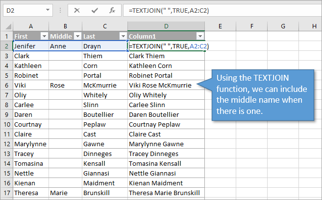
The TEXTJOIN function has three arguments.
- The first argument is delimiter. This is the character (or string of characters) that you want to appear between the text in your cells. In our example of names, we want them separated by a space, so we type ” “.
- The second argument is for ignoring empty cells. You choose either true or false, depending on if you want Excel to disregard cells that are blank. We do, so we will type TRUE.
- The third argument is text. These are the cells you want to combine. You can select them individually, or select an entire range.
All together, our formula is written: =TEXTJOIN(” “,TRUE,A2:C2)
3. Power Query
Compatibility: Excel 2010 or later for Windows
The Merge Columns feature of Power Query is another great way to quickly combine multiple columns and add a separator character.
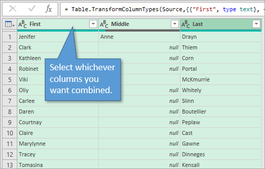
- To combine the contents of cells using Power Query, start by going to the Data tab (Power Query tab for older versions of Excel).
- Choose the option that says From Sheet or From Table or Range (depending on your version). That will open up a preview of your data in the Power Query Editor.
- Select the columns that you want to combine.
- Then select Merge Columns on the Add Column tab. That will bring up the Merge Columns Window.
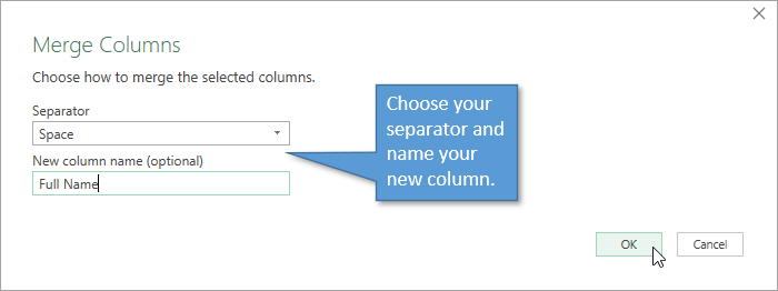
- Select your choice for how you want the text from each column to be separated. In our case, we want a space between the names.
- You can also name the column from this window.
- Hit OK.
A new column with the merged text will be added to the preview.
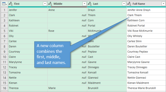
Power Query automatically detects and skips over any blank (null) cells when it combines the columns.
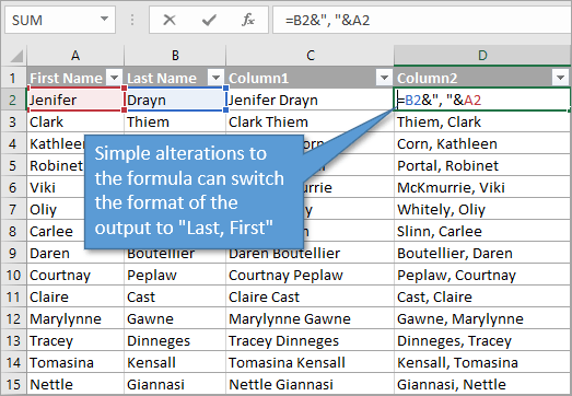
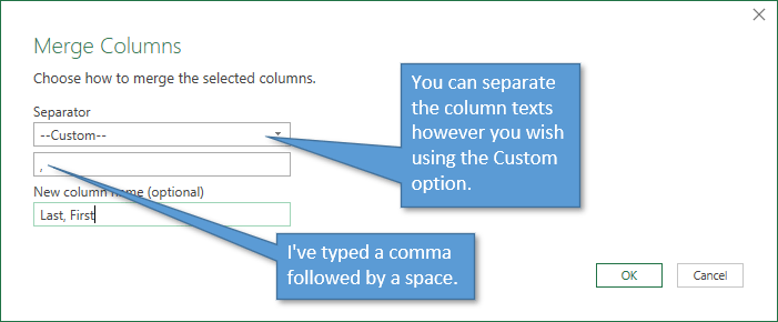
If you instead wanted the format to be “Last, First” in your merged column, the process is similar. The order in which you select your columns before selecting Merge Columns is the same order that they will appear in the output. Instead of selecting Space for your Separator, choose Custom, and then type a comma and a space.
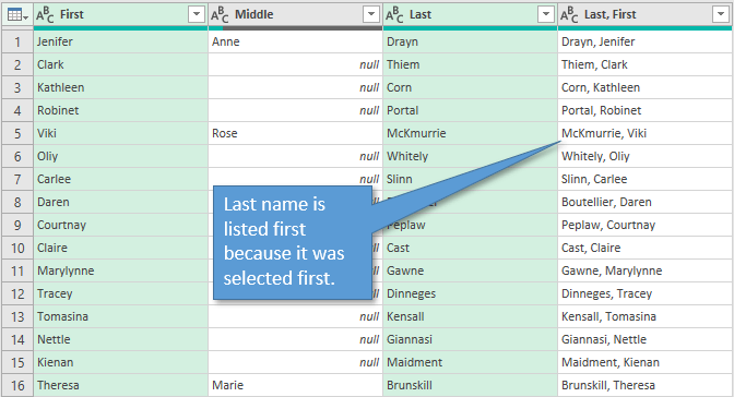
When you hit OK, the new merged column will appear with the desired format.
If your preview looks the way you want it to, you can click on the top half of the Close & Load button to export it into your worksheet.

Note: This process I've described adds your new column to the existing columns on the output sheet. If you want to replace them instead, you simply choose the Merge Columns option on the Transform tab instead of the one on the Add Column tab.
If you're new to Power Query, here is a guide to installing Power Query if you are on an older version of Excel. And check out my free webinar below to learn how to get started with Power Query and the other modern Excel tools/features.
Source: www.excelcampus.com